Load the R package we will use.

library(tidyverse)
library(infer)
library(skimr)

Replace all the instances of ???. These are answers on your moodle quiz.
Run all the individual code chunks to make sure the answers in this file correspond with your quiz answers
After you check all your code chunks run then you can knit it. It won’t knit until the ??? are replaced
Save a plot to be your preview plot

Question: t-test

The data this quiz is a subset of HR
- Look at the variable definitions
- Note that the variables evaluation and salary have been recoded to be represented as words instead of numbers
Set random seed generator to 123 set.seed(123) hr_3_tidy.csv is the name of your data subset
Read it into and assign to hr
- Note: col_types = “fddfff” defines the column types factor-double-double-factor-factor-factor

hr  <- read_csv("https://estanny.com/static/week13/data/hr_3_tidy.csv", 
                col_types = "fddfff")

use the skim to summarize the data in hr

skim(hr)

Table 1: Data summary
Name	hr
Number of rows	500
Number of columns	6
_______________________
Column type frequency:
factor	4
numeric	2
________________________
Group variables	None

Variable type: factor

skim_variable	complete_rate	ordered	n_unique	top_counts
gender	1	FALSE	2	fem: 253, mal: 247
evaluation	1	FALSE	4	bad: 148, fai: 138, goo: 122, ver: 92
salary	1	FALSE	6	lev: 98, lev: 87, lev: 87, lev: 86
status	1	FALSE	3	fir: 196, pro: 172, ok: 132

Variable type: numeric

skim_variable	n_missing	complete_rate	mean	sd	p0	p25	p50	p75	p100	hist
age	0	1	39.41	11.33	20	29.9	39.35	49.1	59.9	▇▇▇▇▆
hours	0	1	49.68	13.24	35	38.2	45.50	58.8	79.9	▇▃▃▂▂

The mean hours worked per week is: 49.7

#Q: Is the mean number of hours worked per week 48? specify that hours is the variable of interest

hr  %>% 
  specify(response = hours)

Response: hours (numeric)
# A tibble: 500 x 1
   hours
   <dbl>
 1  49.6
 2  39.2
 3  63.2
 4  42.2
 5  54.7
 6  54.3
 7  37.3
 8  45.6
 9  35.1
10  53  
# … with 490 more rows

hypothesize that the average hours worked is 48

hr  %>% 
  specify(response = hours)  %>% 
  hypothesize(null = "point", mu = 48)

Response: hours (numeric)
Null Hypothesis: point
# A tibble: 500 x 1
   hours
   <dbl>
 1  49.6
 2  39.2
 3  63.2
 4  42.2
 5  54.7
 6  54.3
 7  37.3
 8  45.6
 9  35.1
10  53  
# … with 490 more rows

#generate 1000 replicates representing the null hypothesis

hr %>% 
  specify(response = hours)  %>% 
  hypothesize(null = "point", mu = 48)  %>% 
  generate(reps = 1000, type = "bootstrap")

Response: hours (numeric)
Null Hypothesis: point
# A tibble: 500,000 x 2
# Groups:   replicate [1,000]
   replicate hours
       <int> <dbl>
 1         1  35.0
 2         1  57.4
 3         1  52.7
 4         1  47.8
 5         1  69.7
 6         1  33.6
 7         1  68.5
 8         1  59.0
 9         1  41.2
10         1  36.9
# … with 499,990 more rows

The output has 500,000 rows

#calculate the distribution of statistics from the generated data - Assign the output null_t_distribution - Display null_t_distribution

null_t_distribution  <- hr  %>% 
  specify(response = age)  %>% 
  hypothesize(null = "point", mu = 48)  %>% 
  generate(reps = 1000, type = "bootstrap")  %>% 
  calculate(stat = "t")

null_t_distribution

# A tibble: 1,000 x 2
   replicate   stat
 *     <int>  <dbl>
 1         1  0.687
 2         2  0.464
 3         3  1.58 
 4         4  1.05 
 5         5 -0.453
 6         6  1.01 
 7         7  2.51 
 8         8 -1.15 
 9         9  1.41 
10        10 -0.292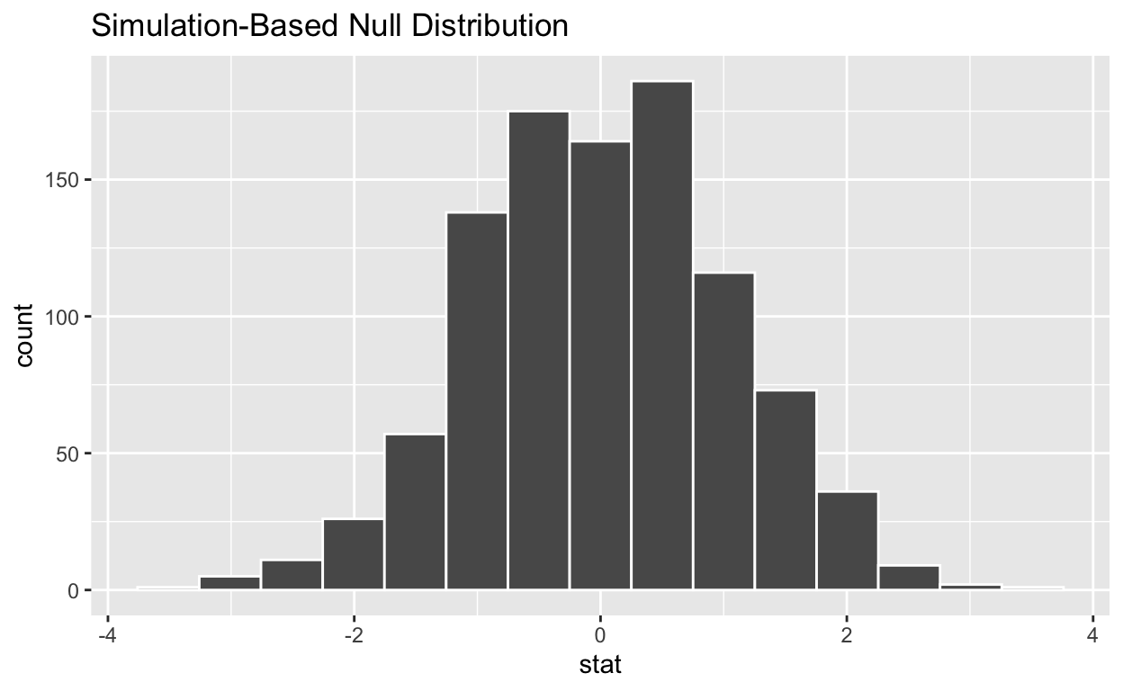
# … with 990 more rows

null_t_distribution has 1,000 t-stats

#visualize the simulated null distribution

visualize(null_t_distribution)

#calculate the statistic from your observed data - Assign the output observed_t_statistic - Display observed_t_statistic

observed_t_statistic  <- hr  %>%
  specify(response = hours)  %>% 
  hypothesize(null = "point", mu = 48)  %>%
  calculate(stat = "t")

observed_t_statistic

# A tibble: 1 x 1
   stat
  <dbl>
1  2.83

#get_p_value from the simulated null distribution and the observed statistic

null_t_distribution  %>% 
  get_p_value(obs_stat = observed_t_statistic, direction = "two-sided")

# A tibble: 1 x 1
  p_value
    <dbl>
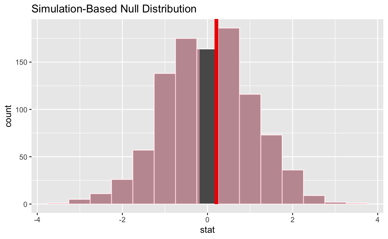
1   0.006

#shade_p_value on the simulated null distribution

null_t_distribution  %>% 
  visualize() +
  shade_p_value(obs_stat = observed_t_statistic, direction = "two-sided")

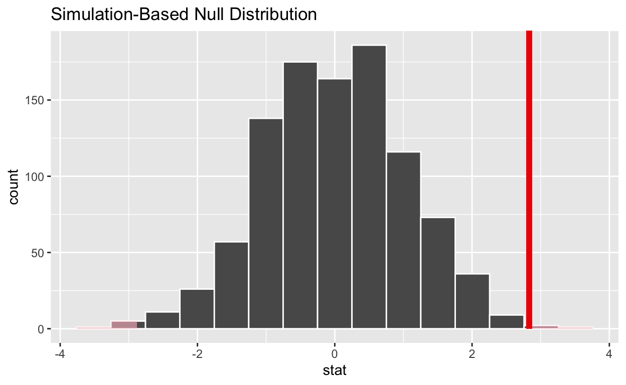
If the p-value < 0.05? yes

Does your analysis support the null hypothesis that the true mean number of hours worked was 48? no

#Question: 2 sample t-test hr_3_tidy.csv is the name of your data subset - Read it into and assign to hr_2 - Note: col_types = “fddfff” defines the column types factor-double-double-factor-factor-factor

hr_2 <- read_csv("https://estanny.com/static/week13/data/hr_3_tidy.csv", 
                col_types = "fddfff")

#Q: Is the average number of hours worked the same for both genders? #use skim to summarize the data in hr_2 by gender

hr_2 %>% 
  group_by(gender)  %>% 
  skim()

Table 2: Data summary
Name	Piped data
Number of rows	500
Number of columns	6
_______________________
Column type frequency:
factor	3
numeric	2
________________________
Group variables	gender

Variable type: factor

skim_variable	gender	complete_rate	ordered	n_unique	top_counts
evaluation	male	1	FALSE	4	bad: 72, fai: 67, goo: 61, ver: 47
evaluation	female	1	FALSE	4	bad: 76, fai: 71, goo: 61, ver: 45
salary	male	1	FALSE	6	lev: 47, lev: 43, lev: 43, lev: 42
salary	female	1	FALSE	6	lev: 51, lev: 46, lev: 45, lev: 43
status	male	1	FALSE	3	fir: 98, pro: 81, ok: 68
status	female	1	FALSE	3	fir: 98, pro: 91, ok: 64

Variable type: numeric

skim_variable	gender	complete_rate	mean	sd	p0	p25	p50	p75	p100	hist
age	male	1	38.23	10.86	20	28.9	37.9	47.05	59.9	▇▇▇▇▅
age	female	1	40.56	11.67	20	31.0	40.3	50.50	59.8	▆▆▇▆▇
hours	male	1	49.55	13.11	35	38.4	45.4	57.65	79.9	▇▃▂▂▂
hours	female	1	49.80	13.38	35	38.2	45.6	59.40	79.8	▇▂▃▂▂

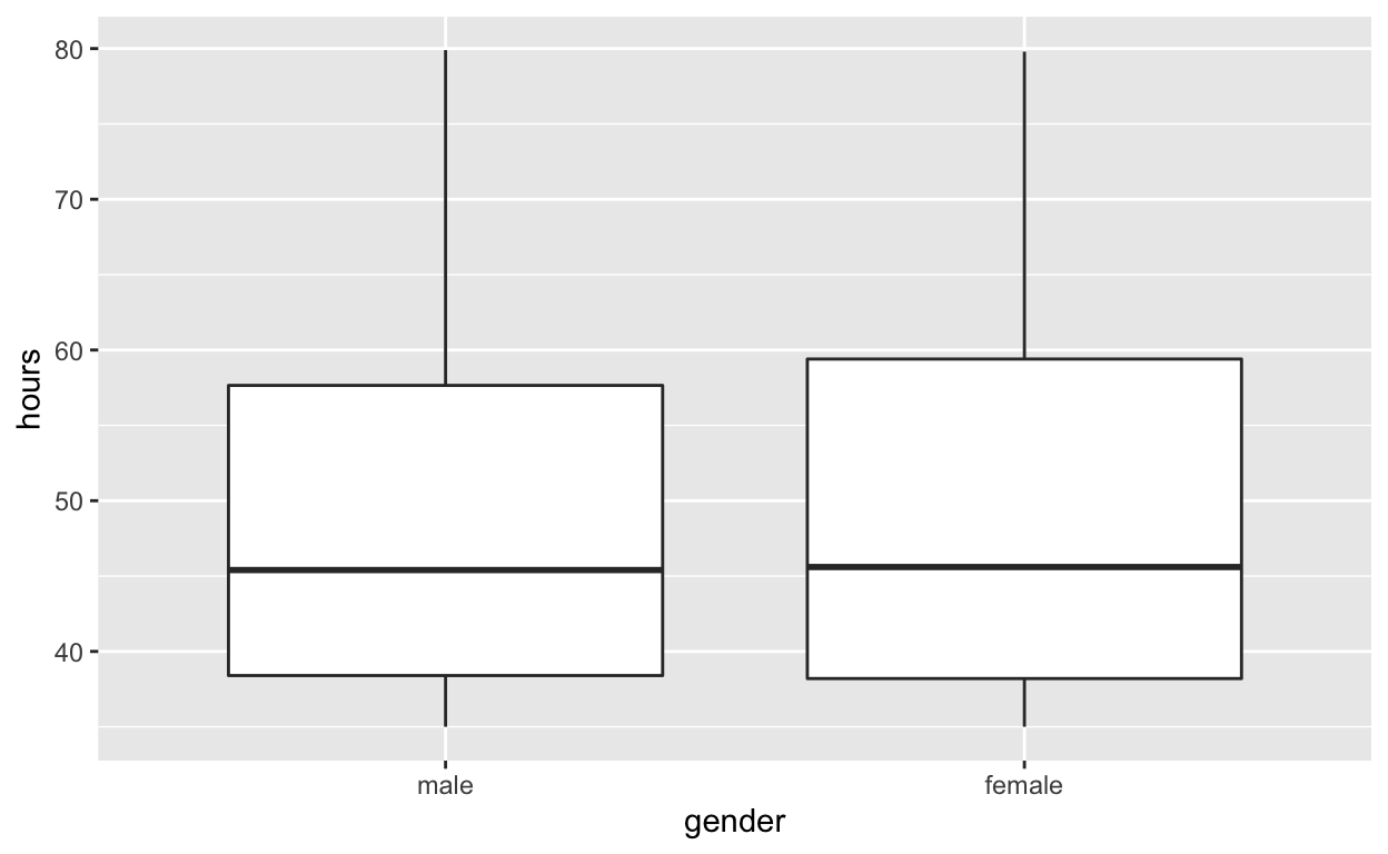
Females worked an average of 49.8 hours per week
Males worked an average of 49.6 hours per week

#Use geom_boxplot to plot distributions of hours worked by gender

hr_2 %>% 
  ggplot(aes(x = gender, y = hours)) + 
  geom_boxplot()

#Specify the variables of interest are hours and gender

hr_2 %>% 
  specify(response = hours, explanatory = gender)

Response: hours (numeric)
Explanatory: gender (factor)
# A tibble: 500 x 2
   hours gender
   <dbl> <fct> 
 1  49.6 male  
 2  39.2 female
 3  63.2 female
 4  42.2 male  
 5  54.7 male  
 6  54.3 female
 7  37.3 female
 8  45.6 female
 9  35.1 female
10  53   male  
# … with 490 more rows

#Hypothesize that the number of hours worked and gender are independent

hr_2  %>% 
  specify(response = hours, explanatory = gender)  %>% 
  hypothesize(null = "independence")

Response: hours (numeric)
Explanatory: gender (factor)
Null Hypothesis: independence
# A tibble: 500 x 2
   hours gender
   <dbl> <fct> 
 1  49.6 male  
 2  39.2 female
 3  63.2 female
 4  42.2 male  
 5  54.7 male  
 6  54.3 female
 7  37.3 female
 8  45.6 female
 9  35.1 female
10  53   male  
# … with 490 more rows

#Generate 1000 replicates representing the null hypothesis

hr_2 %>% 
  specify(response = hours, explanatory = gender)  %>% 
  hypothesize(null = "independence")  %>% 
  generate(reps = 1000, type = "permute")

Response: hours (numeric)
Explanatory: gender (factor)
Null Hypothesis: independence
# A tibble: 500,000 x 3
# Groups:   replicate [1,000]
   hours gender replicate
   <dbl> <fct>      <int>
 1  45.1 male           1
 2  63.8 female         1
 3  46.1 female         1
 4  39.9 male           1
 5  51.6 male           1
 6  56.6 female         1
 7  42.1 female         1
 8  35.3 female         1
 9  73.6 female         1
10  35.8 male           1
# … with 499,990 more rows

The output has 500,000 rows

#Calculate the distribution of statistics from the generated data - Assign the output null_distribution_2_sample_permute - Display null_distribution_2_sample_permute

null_distribution_2_sample_permute  <- hr_2 %>% 
  specify(response = hours, explanatory = gender)  %>% 
  hypothesize(null = "independence")  %>% 
  generate(reps = 1000, type = "permute")  %>% 
  calculate(stat = "t", order = c("female", "male"))

null_distribution_2_sample_permute

# A tibble: 1,000 x 2
   replicate      stat
 *     <int>     <dbl>
 1         1 -0.872   
 2         2  0.560   
 3         3 -0.0900  
 4         4 -1.14    
 5         5 -0.779   
 6         6 -0.314   
 7         7 -0.592   
 8         8  1.28    
 9         9  0.828   
10        10  0.000502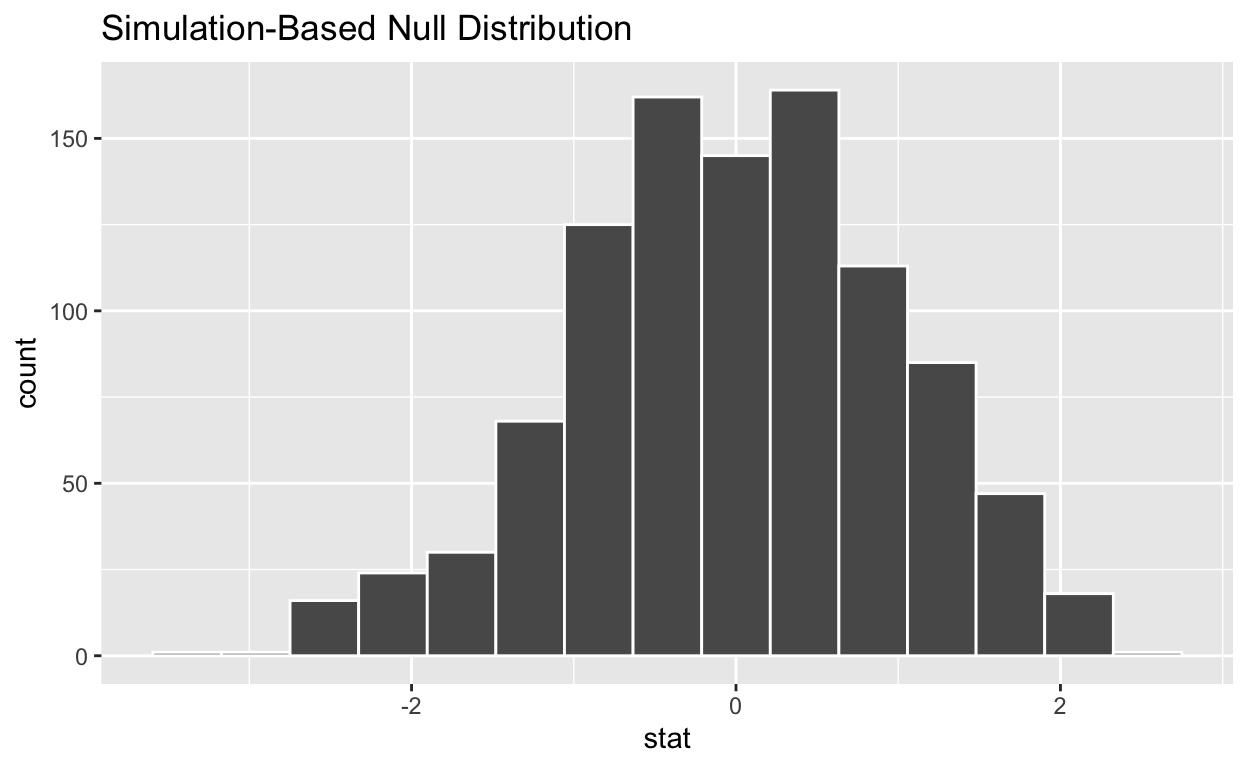
# … with 990 more rows

null_t_distribution has ??? t-stats

#Visualize the simulated null distribution

visualize(null_distribution_2_sample_permute)

#Calculate the statistic from your observed data - Assign the output observed_t_2_sample_stat - Display observed_t_2_sample_stat

observed_t_2_sample_stat  <- hr_2 %>%
  specify(response = hours, explanatory = gender)  %>% 
  calculate(stat = "t", order = c("female", "male"))

observed_t_2_sample_stat

# A tibble: 1 x 1
   stat
  <dbl>
1 0.208

#Get_p_value from the simulated null distribution and the observed statistic

null_t_distribution  %>% 
  get_p_value(obs_stat = observed_t_2_sample_stat, direction = "two-sided")

# A tibble: 1 x 1
  p_value
    <dbl>
1   0.872

#Shade_p_value on the simulated null distribution

null_t_distribution  %>% 
  visualize() +
  shade_p_value(obs_stat = observed_t_2_sample_stat, direction = "two-sided")

If the p-value < 0.05? no

Does your analysis support the null hypothesis that the true mean number of hours worked by female and male employees was the same? yes

#Question: ANOVA hr_1_tidy.csv is the name of your data subset - Read it into and assign to hr_anova - Note: col_types = “fddfff” defines the column types factor-double-double-factor-factor-factor

hr_anova <- read_csv("https://estanny.com/static/week13/data/hr_1_tidy.csv", 
                col_types = "fddfff")

#Q: Is the average number of hours worked the same for all three status (fired, ok and promoted) ? use skim to summarize the data in hr_anova by status

hr_anova %>% 
  group_by(status)  %>% 
  skim()

Table 3: Data summary
Name	Piped data
Number of rows	500
Number of columns	6
_______________________
Column type frequency:
factor	3
numeric	2
________________________
Group variables	status

Variable type: factor

skim_variable	status	complete_rate	ordered	n_unique	top_counts
gender	fired	1	FALSE	2	fem: 96, mal: 89
gender	ok	1	FALSE	2	fem: 77, mal: 76
gender	promoted	1	FALSE	2	fem: 87, mal: 75
evaluation	fired	1	FALSE	4	bad: 65, fai: 63, goo: 31, ver: 26
evaluation	ok	1	FALSE	4	bad: 69, fai: 59, goo: 15, ver: 10
evaluation	promoted	1	FALSE	4	ver: 63, goo: 60, fai: 20, bad: 19
salary	fired	1	FALSE	6	lev: 41, lev: 37, lev: 32, lev: 32
salary	ok	1	FALSE	6	lev: 40, lev: 37, lev: 29, lev: 23
salary	promoted	1	FALSE	6	lev: 37, lev: 35, lev: 29, lev: 23

Variable type: numeric

skim_variable	status	complete_rate	mean	sd	p0	p25	p50	p75	p100	hist
age	fired	1	38.64	11.43	20.2	28.30	38.30	47.60	59.6	▇▇▇▅▆
age	ok	1	41.34	12.11	20.3	31.00	42.10	51.70	59.9	▆▆▆▆▇
age	promoted	1	42.13	10.98	21.0	33.40	42.95	50.98	59.9	▆▅▆▇▇
hours	fired	1	41.67	7.88	35.0	36.10	38.90	43.90	75.5	▇▂▁▁▁
hours	ok	1	48.05	11.65	35.0	37.70	45.60	56.10	78.2	▇▃▃▂▁
hours	promoted	1	59.27	12.90	35.0	51.12	60.10	70.15	79.7	▆▅▇▇▇

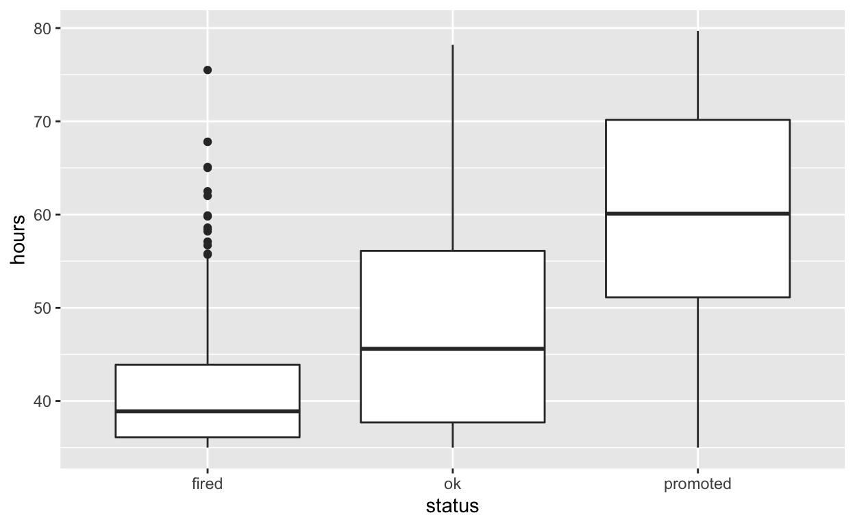
Employees that were fired worked an average of 41.7 hours per week
Employees that were ok worked an average of 48.0 hours per week
Employees that were promoted worked an average of 59.3 hours per week

#Use geom_boxplot to plot distributions of hours worked by status

hr_anova %>% 
  ggplot(aes(x = status, y = hours)) + 
  geom_boxplot()

#Specify the variables of interest are hours and status

hr_anova %>% 
  specify(response = hours, explanatory = status)

Response: hours (numeric)
Explanatory: status (factor)
# A tibble: 500 x 2
   hours status  
   <dbl> <fct>   
 1  36.5 fired   
 2  55.8 ok      
 3  35   fired   
 4  52   promoted
 5  35.1 ok      
 6  36.3 ok      
 7  40.1 promoted
 8  42.7 fired   
 9  66.6 promoted
10  35.5 ok      
# … with 490 more rows

#Hypothesize that the number of hours worked and status are independent

hr_anova  %>% 
  specify(response = hours, explanatory = status)  %>% 
  hypothesize(null = "independence")

Response: hours (numeric)
Explanatory: status (factor)
Null Hypothesis: independence
# A tibble: 500 x 2
   hours status  
   <dbl> <fct>   
 1  36.5 fired   
 2  55.8 ok      
 3  35   fired   
 4  52   promoted
 5  35.1 ok      
 6  36.3 ok      
 7  40.1 promoted
 8  42.7 fired   
 9  66.6 promoted
10  35.5 ok      
# … with 490 more rows

#Generate 1000 replicates representing the null hypothesis

hr_anova %>% 
  specify(response = hours, explanatory = status)  %>% 
  hypothesize(null = "independence")  %>% 
  generate(reps = 1,000, type = "permute")

Response: hours (numeric)
Explanatory: status (factor)
Null Hypothesis: independence
# A tibble: 500 x 3
# Groups:   replicate [1]
   hours status   replicate
   <dbl> <fct>        <int>
 1  71.3 fired            1
 2  73.7 ok               1
 3  61.4 fired            1
 4  55.8 promoted         1
 5  35.4 ok               1
 6  50.1 ok               1
 7  38   promoted         1
 8  50.7 fired            1
 9  76.3 promoted         1
10  55.7 ok               1
# … with 490 more rows

The output has 500 rows

#Calculate the distribution of statistics from the generated data - Assign the output null_distribution_anova - Display null_distribution_anova

null_distribution_anova  <- hr_anova %>% 
  specify(response = hours, explanatory = gender)  %>% 
  hypothesize(null = "independence")  %>% 
  generate(reps = 1000, type = "permute")  %>% 
  calculate(stat = "F")

null_distribution_anova

# A tibble: 1,000 x 2
   replicate   stat
 *     <int>  <dbl>
 1         1 0.789 
 2         2 0.110 
 3         3 0.727 
 4         4 2.39  
 5         5 0.0832
 6         6 0.146 
 7         7 0.118 
 8         8 0.309 
 9         9 0.434 
10        10 1.74  
# … with 990 more rows

null_distribution_anova has 1,000 F-stats

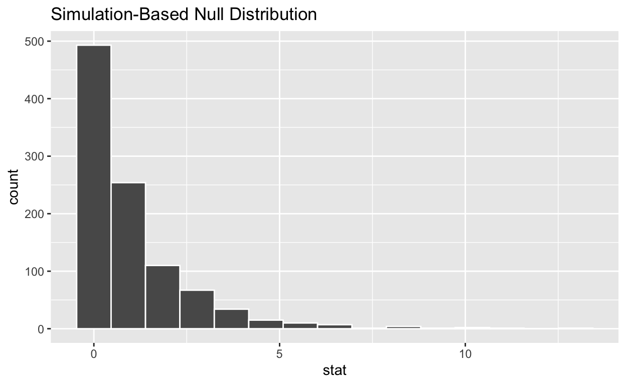
#Visualize the simulated null distribution

visualize(null_distribution_anova)

#Calculate the statistic from your observed data - Assign the output observed_f_sample_stat - Display observed_f_sample_stat

observed_f_sample_stat  <- hr_anova %>%
  specify(response = hours, explanatory = status)  %>% 
  calculate(stat = "F")

observed_f_sample_stat

# A tibble: 1 x 1
   stat
  <dbl>
1  115.

#Get_p_value from the simulated null distribution and the observed statistic

null_distribution_anova  %>% 
  get_p_value(obs_stat = observed_f_sample_stat, direction = "greater")

# A tibble: 1 x 1
  p_value
    <dbl>
1       0

#Shade_p_value on the simulated null distribution

null_t_distribution  %>% 
  visualize() +
  shade_p_value(obs_stat = observed_f_sample_stat, direction = "greater")

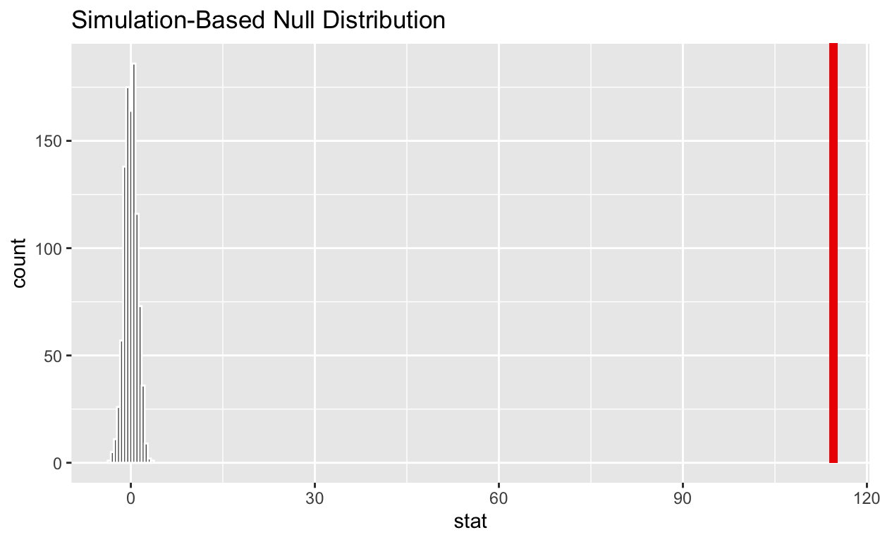
If the p-value < 0.05? yes

Does your analysis support the null hypothesis that the true means of the number of hours worked for those that were “fired”, “ok” and “promoted” were the same? no

Hypothesis Testing

Question: t-test

use the skim to summarize the data in hr